DIVEIN

Divergence, Diversity,
Informative Sites and
Phylogenetic Analyses
Informative Sites and
Phylogenetic Analyses
The input nucleotide or amino-acid sequences must be aligned. DIVEIN accepts two types of sequence files, which are fasta and phylip. The sequence data set could be in either sequential or interleaved format. The name of sequences MUST NOT contain any whitespace characters (tab or space). It is recommended that the sequence name is comprised of alphabetical characters, digits or underscore. The program will replace any other characters with underscore "_".
Example of phylip file in sequential format:
12 150
092398_316    GAAGAAGAGGTAATAATTAGATCACAGAATTTCACGGACAATGCTAAAACCATATTAGTACAGCTGAATGAAACTGTACAAATTAATTGTACAAGACCCAACAACAATACAAGAAAAAGCATACATATAGCACCAGGGAGAGCATTTTAT
092398_339    GAAGAAGAGGTAATAATTAGATCACAGAATTTCACGGACAATGCTAAAACCATATTAGTACAGCTGAATGAAACTGTACAAATTAATTGTACAAGACCCAACAACAATACAAGAAAAAGCATACATATAGCACCAGGGAGAGCATTTTAT
092398_315    GAAGAAGAGGTAATAATTAGATCACAGAATTTCACGGACAATGCTAAAACCATATTAGTACAGCTGAATGAAACTGTACAAATTAATTGTACAAGACCCAACAACAATACAAGAAAAAGCATACATATAGCACCAGGGAGAGCATTTTAT
092398_317    GAAGAAGAGGTAATAATTAGATCACAGAATTTCACGGACAATGCTAAAACCATATTAGTACAGCTGAATGAAACTGTACAAATTAATTGTACAAGACCCAACAACAATACAAGAAAAAGCATACATATAGCACCAGGGAGAGCATTTTAT
092398_312    GAAGAAGAGGTAATAATTAGATCACAGAATTTCACGGACAATGCTAAAACCATATTAGTACAGCTGAATGAAACTGTACAAATTAATTGTACAAGACCCAACAACAATACAAGAAAAAGCATACATATAGCACCAGGGAGAGCATTTTAT
082599_889    GAAGAAGAGGTAATAATTAGATCACAGAATTTCACGGACAATGCTAAAACCATATTAGTACAGCTGAATGAAACTGTACAAATTAATTGTACAAGACTCAACAACAATACAAGAAAAAGCATACATATAGCACCAGGGAGAGCATTTTAT
082599_894    GAAGAAGAGGTAATAATTAGATCACAGAATTTCACGGACAATGCCAAAACCATATTAGTACAGCTGAATGAAACTGTACAAATTAATTGTACAAGACCCAACGACAATACAAGAAAAAGCATACATATAGCACCAGGGAGAGCATTTTAT
082599_896    GAAGAAGAGGTAATAATTAGATCACAGAATTTCACGGACAATGCTAAAACCATATTAGTACAGCTGAATGAAACTGTACAAATTAATTGTACAAGACCCAACAACAATACAAGAAAAAGCATACATATAGCACCAGGGAGAGCATTTTAT
082599_916    GAAGAAGAGGTAATAATTAGATCACAGAATTTCACGGACAATGCTAAAACCATATTAGTACAGCTGAATGAAACTGTACAAATTAATTGTACAAGACCCAACAACAATACAAGAAAAAGCATACATATAGCACCAGGGAGAGCATTTTAT
082599_917    GAAGAAGAGGTAATAATTAGATCACAGAATTTCACGGACAATGCTAAAACCATATTAGTACAGCTGAATGAAACTGTACAAATTAATTGTACAAGACCCAACAACAATACAAGAAAAAGCATACATATAGCACCAGGGAGAGCATTTTAT
ML1365_1      GAAGAAGAGGTAATAATTAGATCACAAAATTTCACAGACAATGCTAAAACCATATTAGTACAGCTGAATGAAACTGTACAAATTAATTGTACAAGACCCAACAACAATACAAGAAAAAGCATACATATAGCACCAGGGAGAGCATTTTAT
ML1365_2      GAAGAAGAGGTAATAATTAGATCACAAAATTTCACAGACAATGCTAAAACCATATTAGTACAGCTGAATGAAACTGTACAAATTAATTGTACAAGACCCAACAACAATACAAGAAAAAGCATACATATAGCACCAGGGAGAGCATTTTAT
Example of phylip file in interleaved format:
12 150
092398_316    GAAGAAGAGGTAATAATTAGATCACAGAATTTCACGGACAATGCTAAAACCATATTAGTACAGCTGAATGAAACTGTACA
092398_339    GAAGAAGAGGTAATAATTAGATCACAGAATTTCACGGACAATGCTAAAACCATATTAGTACAGCTGAATGAAACTGTACA
092398_315    GAAGAAGAGGTAATAATTAGATCACAGAATTTCACGGACAATGCTAAAACCATATTAGTACAGCTGAATGAAACTGTACA
092398_317    GAAGAAGAGGTAATAATTAGATCACAGAATTTCACGGACAATGCTAAAACCATATTAGTACAGCTGAATGAAACTGTACA
092398_312    GAAGAAGAGGTAATAATTAGATCACAGAATTTCACGGACAATGCTAAAACCATATTAGTACAGCTGAATGAAACTGTACA
082599_889    GAAGAAGAGGTAATAATTAGATCACAGAATTTCACGGACAATGCTAAAACCATATTAGTACAGCTGAATGAAACTGTACA
082599_894    GAAGAAGAGGTAATAATTAGATCACAGAATTTCACGGACAATGCCAAAACCATATTAGTACAGCTGAATGAAACTGTACA
082599_896    GAAGAAGAGGTAATAATTAGATCACAGAATTTCACGGACAATGCTAAAACCATATTAGTACAGCTGAATGAAACTGTACA
082599_916    GAAGAAGAGGTAATAATTAGATCACAGAATTTCACGGACAATGCTAAAACCATATTAGTACAGCTGAATGAAACTGTACA
082599_917    GAAGAAGAGGTAATAATTAGATCACAGAATTTCACGGACAATGCTAAAACCATATTAGTACAGCTGAATGAAACTGTACA
ML1365_1      GAAGAAGAGGTAATAATTAGATCACAAAATTTCACAGACAATGCTAAAACCATATTAGTACAGCTGAATGAAACTGTACA
ML1365_2      GAAGAAGAGGTAATAATTAGATCACAAAATTTCACAGACAATGCTAAAACCATATTAGTACAGCTGAATGAAACTGTACA

AATTAATTGTACAAGACCCAACAACAATACAAGAAAAAGCATACATATAGCACCAGGGAGAGCATTTTAT
AATTAATTGTACAAGACCCAACAACAATACAAGAAAAAGCATACATATAGCACCAGGGAGAGCATTTTAT
AATTAATTGTACAAGACCCAACAACAATACAAGAAAAAGCATACATATAGCACCAGGGAGAGCATTTTAT
AATTAATTGTACAAGACCCAACAACAATACAAGAAAAAGCATACATATAGCACCAGGGAGAGCATTTTAT
AATTAATTGTACAAGACCCAACAACAATACAAGAAAAAGCATACATATAGCACCAGGGAGAGCATTTTAT
AATTAATTGTACAAGACTCAACAACAATACAAGAAAAAGCATACATATAGCACCAGGGAGAGCATTTTAT
AATTAATTGTACAAGACCCAACGACAATACAAGAAAAAGCATACATATAGCACCAGGGAGAGCATTTTAT
AATTAATTGTACAAGACCCAACAACAATACAAGAAAAAGCATACATATAGCACCAGGGAGAGCATTTTAT
AATTAATTGTACAAGACCCAACAACAATACAAGAAAAAGCATACATATAGCACCAGGGAGAGCATTTTAT
AATTAATTGTACAAGACCCAACAACAATACAAGAAAAAGCATACATATAGCACCAGGGAGAGCATTTTAT
AATTAATTGTACAAGACCCAACAACAATACAAGAAAAAGCATACATATAGCACCAGGGAGAGCATTTTAT
AATTAATTGTACAAGACCCAACAACAATACAAGAAAAAGCATACATATAGCACCAGGGAGAGCATTTTAT
Example of fasta file:
>092398_316
GAAGAAGAGGTAATAATTAGATCACAGAATTTCACGGACAATGCTAAAACCATATTAGTACAGCTGAATGAAACTGTACA
AATTAATTGTACAAGACCCAACAACAATACAAGAAAAAGCATACATATAGCACCAGGGAGAGCATTTTAT
>092398_339
GAAGAAGAGGTAATAATTAGATCACAGAATTTCACGGACAATGCTAAAACCATATTAGTACAGCTGAATGAAACTGTACA
AATTAATTGTACAAGACCCAACAACAATACAAGAAAAAGCATACATATAGCACCAGGGAGAGCATTTTAT
>092398_315
GAAGAAGAGGTAATAATTAGATCACAGAATTTCACGGACAATGCTAAAACCATATTAGTACAGCTGAATGAAACTGTACA
AATTAATTGTACAAGACCCAACAACAATACAAGAAAAAGCATACATATAGCACCAGGGAGAGCATTTTAT
>092398_317
GAAGAAGAGGTAATAATTAGATCACAGAATTTCACGGACAATGCTAAAACCATATTAGTACAGCTGAATGAAACTGTACA
AATTAATTGTACAAGACCCAACAACAATACAAGAAAAAGCATACATATAGCACCAGGGAGAGCATTTTAT
>092398_312
GAAGAAGAGGTAATAATTAGATCACAGAATTTCACGGACAATGCTAAAACCATATTAGTACAGCTGAATGAAACTGTACA
AATTAATTGTACAAGACCCAACAACAATACAAGAAAAAGCATACATATAGCACCAGGGAGAGCATTTTAT
>082599_889
GAAGAAGAGGTAATAATTAGATCACAGAATTTCACGGACAATGCTAAAACCATATTAGTACAGCTGAATGAAACTGTACA
AATTAATTGTACAAGACTCAACAACAATACAAGAAAAAGCATACATATAGCACCAGGGAGAGCATTTTAT
>082599_894
GAAGAAGAGGTAATAATTAGATCACAGAATTTCACGGACAATGCCAAAACCATATTAGTACAGCTGAATGAAACTGTACA
AATTAATTGTACAAGACCCAACGACAATACAAGAAAAAGCATACATATAGCACCAGGGAGAGCATTTTAT
>082599_896
GAAGAAGAGGTAATAATTAGATCACAGAATTTCACGGACAATGCTAAAACCATATTAGTACAGCTGAATGAAACTGTACA
AATTAATTGTACAAGACCCAACAACAATACAAGAAAAAGCATACATATAGCACCAGGGAGAGCATTTTAT
>082599_916
GAAGAAGAGGTAATAATTAGATCACAGAATTTCACGGACAATGCTAAAACCATATTAGTACAGCTGAATGAAACTGTACA
AATTAATTGTACAAGACCCAACAACAATACAAGAAAAAGCATACATATAGCACCAGGGAGAGCATTTTAT
>082599_917
GAAGAAGAGGTAATAATTAGATCACAGAATTTCACGGACAATGCTAAAACCATATTAGTACAGCTGAATGAAACTGTACA
AATTAATTGTACAAGACCCAACAACAATACAAGAAAAAGCATACATATAGCACCAGGGAGAGCATTTTAT
>ML1365_1
GAAGAAGAGGTAATAATTAGATCACAAAATTTCACAGACAATGCTAAAACCATATTAGTACAGCTGAATGAAACTGTACA
AATTAATTGTACAAGACCCAACAACAATACAAGAAAAAGCATACATATAGCACCAGGGAGAGCATTTTAT
>ML1365_2
GAAGAAGAGGTAATAATTAGATCACAAAATTTCACAGACAATGCTAAAACCATATTAGTACAGCTGAATGAAACTGTACA
AATTAATTGTACAAGACCCAACAACAATACAAGAAAAAGCATACATATAGCACCAGGGAGAGCATTTTAT
DNA or amino-acid. You must select correct data type for your sequence alignment file.
2. Informative Sites
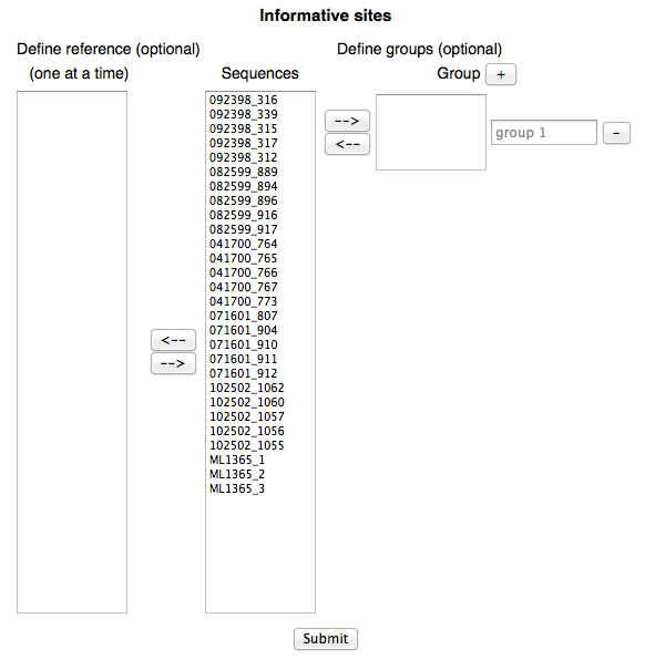
From the interface above user has options to define a reference sequence and/or group(s) of sequences of his wish. If a reference sequence is defined, DIVEIN will use it to detect informative and private sites in the alignment. If there is no reference sequence defined, DIVEIN will calculate the consensus sequence and use it as a reference to detect informative sites. If sequence group(s) are defined, DIVEIN will calculate informative sites based on each group.
2.2 Outputs
Aligned informative sites: An output file where all detected informative sites are aligned.
Example of aligned informative sites:
                1334579
               85120394

Consensus      CGGGGGAA
Dec03_1        ....T..C
Dec03_2        ....TAC.
Dec03_3        ........
Dec03_4        GA......
Dec03_5        GA......
Mar04_1        ....T..C
Mar04_2        G.TT....
Mar04_7        .....AC.
Mar04_8        ........
Mar04_9        ..TT....
Tab-delimited informative sites & summary: A tab-delimited output file containing all detected informative sites and summary of informative sites.
Example of tab-delimited informative sites & summary:
         	Total_informative	Informative(noGaps)	     	 8	15	31	32	40	53	79	94
Consensus	                0	                  0	     	 C	 G	 G	 G	 G	 G	 A	 A
Dec03_1  	                2	                  2	     	 .	 .	 .	 .	 T	 .	 .	 C
Dec03_2  	                3	                  3	     	 .	 .	 .	 .	 T	 A	 C	 .
Dec03_3  	                0	                  0	     	 .	 .	 .	 .	 .	 .	 .	 .
Dec03_4  	                2	                  2	     	 G	 A	 .	 .	 .	 .	 .	 .
Dec03_5  	                2	                  2	     	 G	 A	 .	 .	 .	 .	 .	 .
Mar04_1  	                2	                  2	     	 .	 .	 .	 .	 T	 .	 .	 C
Mar04_2  	                3	                  3	     	 G	 .	 T	 T	 .	 .	 .	 .
Mar04_7  	                2	                  2	     	 .	 .	 .	 .	 .	 A	 C	 .
Mar04_8  	                0	                  0	     	 .	 .	 .	 .	 .	 .	 .	 .
Mar04_9  	                2	                  2	     	 .	 .	 T	 T	 .	 .	 .	 .

Alignment	                8	                  8
         	                 	                   	    A	 0	 2	 0	 0	 0	 2	 8	 8
         	                 	                   	    C	 7	 0	 0	 0	 0	 0	 2	 2
         	                 	                   	    G	 3	 8	 8	 8	 7	 8	 0	 0
         	                 	                   	    T	 0	 0	 2	 2	 3	 0	 0	 0
         	                 	                   	Total	10	10	10	10	10	10	10	10
Aligned private sites: An output file where all detected private sites are aligned.
Example of aligned private sites:
                359
               5008

Consensus      GGAA
Dec03_1        ....
Dec03_2        ....
Dec03_3        ....
Dec03_4        ....
Dec03_5        ....
Mar04_1        ....
Mar04_2        .C..
Mar04_7        ...G
Mar04_8        A.G.
Mar04_9        .T..
Tab-delimited private sites & summary: A tab-delimited output file containing all detected private sites and summary of private sites.
Example of tab-delimited private sites & summary:
         	Total_private	Private(noGaps)	     	 5	30	50	98
Consensus	            0	              0	     	 G	 G	 A	 A
Dec03_1  	            0	              0	     	 .	 .	 .	 .
Dec03_2  	            0	              0	     	 .	 .	 .	 .
Dec03_3  	            0	              0	     	 .	 .	 .	 .
Dec03_4  	            0	              0	     	 .	 .	 .	 .
Dec03_5  	            0	              0	     	 .	 .	 .	 .
Mar04_1  	            0	              0	     	 .	 .	 .	 .
Mar04_2  	            1	              1	     	 .	 C	 .	 .
Mar04_7  	            1	              1	     	 .	 .	 .	 G
Mar04_8  	            2	              2	     	 A	 .	 G	 .
Mar04_9  	            1	              1	     	 .	 T	 .	 .

Alignment	            4	              4
         	             	               	    A	 1	 0	 9	 9
         	             	               	    C	 0	 1	 0	 0
         	             	               	    G	 9	 8	 1	 1
         	             	               	    T	 0	 1	 0	 0
         	             	               	Total	10	10	10	10
3. Center of Tree
3.1 Inputs
3.2 Outputs
Initial tree:
 COT re-rooted tree:
Users can perform Maximum Likelihood (ML) estimation alone or include divergence/diversity analyses through three programs (FastTree, RAxML and PhyML). They can select to calculate divergence from any or all of: MRCA, COT, consensus, or any sequence in the alignment.
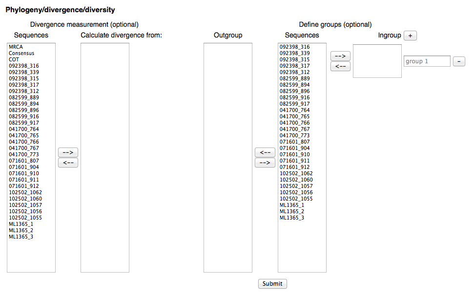
From the interface above, user has options to define one or more sequences to calculate divergence from the defined sequences (MRCA, COT, consensus and any sequences in alignment), and/or to designate sequences into different groups at his wish. If user wants to calculate divergence from MRCA, he has to define outgroup sequence(s). If ingroups are defined, diversity and divergence are calculated based on each ingroup.
When an analysis is finished, a link is sent to the user by email to view and download results. Users can locally visualize and edit phylogenetic trees and dynamically generate and download graphs of distance distribution histograms and divergence and diversity (if applicable). Screen shots of DIVEIN output of phylogeney/divergence/diversity analyses are shown in the figure below.
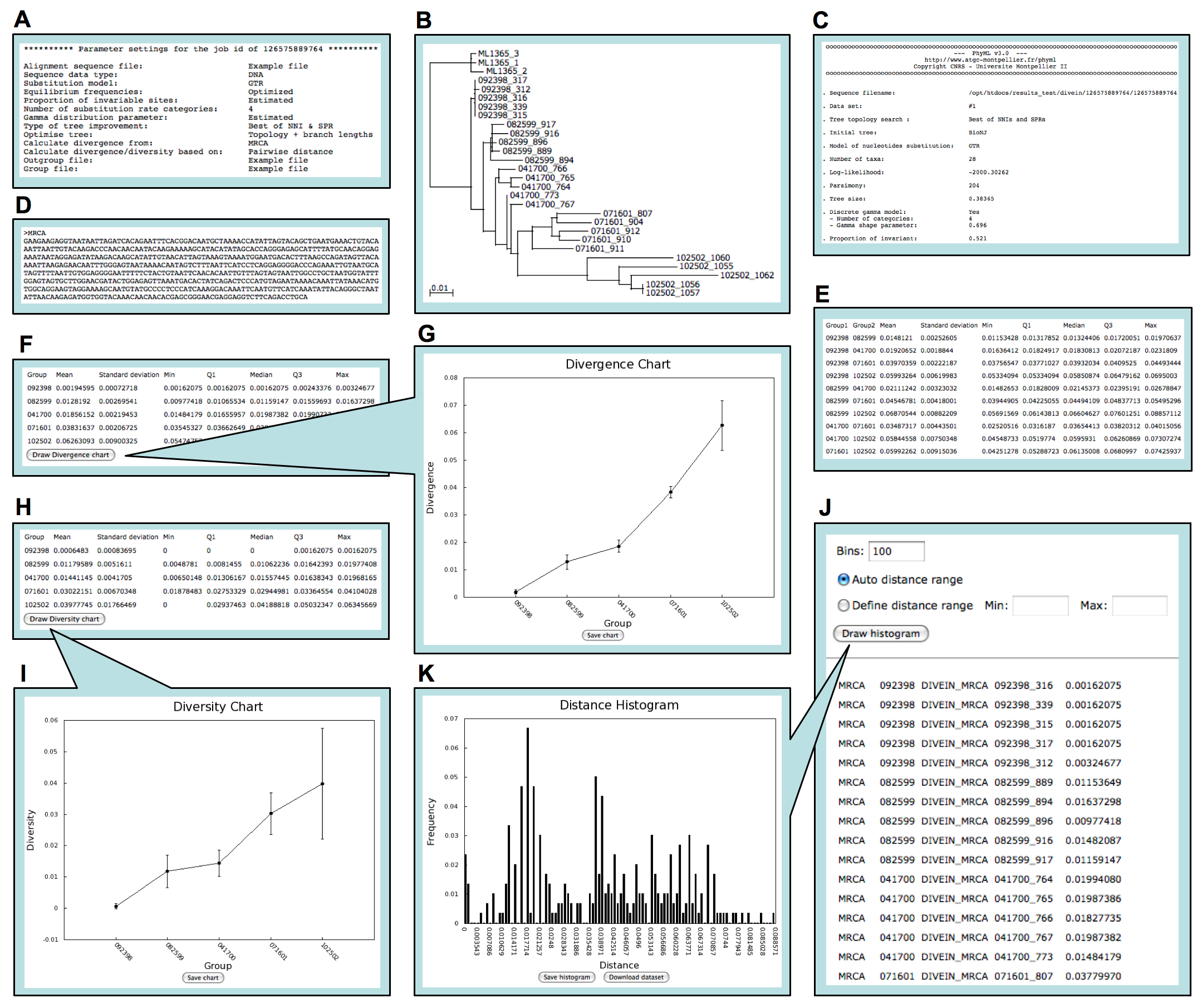
Screen shots of phylogeny/divergence/diversity output in DIVEIN. (A) Parameter settings for running the program. (B) Phylogenetic tree viewed through the Archaeopteryx Java applet. (C) Estimated evolutionary parameters. (D) Reconstructed MRCA sequence. (E) Summarized distances between groups. (F) Summarized divergence from MRCA for each group. (G) Divergence plot generated by clicking the Draw divergence chart button. (H) Summarized diversity for each group. (I) Diversity plot generated by clicking the Draw diversity chart button . (J) Distance matrix. (K) Distance distribution histogram generated by clicking the Draw histogram button.
Example:
sample1	sample1	sample1_1	sample1_2	0.01637381
sample1	sample1	sample1_1	sample1_3	0.00487810
sample1	sample1	sample1_1	sample1_4	0.00980428
sample1	sample1	sample1_1	sample1_5	0.00814550
sample1	sample1	sample1_1	sample1_6	0.01822976
sample1	sample1	sample1_1	sample1_7	0.01970637
sample1	sample1	sample1_1	sample1_8	0.01986091
sample1	sample1	sample1_1	sample1_9	0.02138145
sample1	sample1	sample1_1	sample1_10	0.01637298
sample1	sample1	sample1_2	sample1_3	0.01472954
sample1	sample1	sample1_2	sample1_4	0.01974077
sample1	sample1	sample1_2	sample1_5	0.01807237
sample1	sample1	sample1_2	sample1_6	0.02470691
sample1	sample1	sample1_2	sample1_7	0.02472565
sample1	sample1	sample1_2	sample1_8	0.02635346
sample1	sample1	sample1_2	sample1_9	0.02641488
sample1	sample1	sample1_2	sample1_10	0.02472565
sample1	sample1	sample1_3	sample1_4	0.00815682
sample1	sample1	sample1_3	sample1_5	0.00650614
sample1	sample1	sample1_3	sample1_6	0.01636412
sample1	sample1	sample1_3	sample1_7	0.01803690
sample1	sample1	sample1_3	sample1_8	0.01822346
sample1	sample1	sample1_3	sample1_9	0.01970637
sample1	sample1	sample1_3	sample1_10	0.01478813
sample1	sample1	sample1_4	sample1_5	0.01144043
sample1	sample1	sample1_4	sample1_6	0.02146014
sample1	sample1	sample1_4	sample1_7	0.02309267
sample1	sample1	sample1_4	sample1_8	0.02314722
sample1	sample1	sample1_4	sample1_9	0.02474853
sample1	sample1	sample1_4	sample1_10	0.01982461
sample1	sample1	sample1_5	sample1_6	0.01989424
sample1	sample1	sample1_5	sample1_7	0.02145289
sample1	sample1	sample1_5	sample1_8	0.02150356
sample1	sample1	sample1_5	sample1_9	0.02310453
sample1	sample1	sample1_5	sample1_10	0.01822753
sample1	sample1	sample1_6	sample1_7	0.00814550
sample1	sample1	sample1_6	sample1_8	0.01475515
sample1	sample1	sample1_6	sample1_9	0.01805260
sample1	sample1	sample1_6	sample1_10	0.01472476
sample1	sample1	sample1_7	sample1_8	0.01636654
sample1	sample1	sample1_7	sample1_9	0.01635010
sample1	sample1	sample1_7	sample1_10	0.01634613
sample1	sample1	sample1_8	sample1_9	0.01968165
sample1	sample1	sample1_8	sample1_10	0.01306167
sample1	sample1	sample1_9	sample1_10	0.00650148
sample1	sample2	sample1_1	sample2_1	0.04150894
sample1	sample2	sample1_1	sample2_2	0.04481757
sample1	sample2	sample1_1	sample2_3	0.04118581
sample1	sample2	sample1_1	sample2_4	0.04270911
sample1	sample2	sample1_1	sample2_5	0.04747813
sample1	sample2	sample1_2	sample2_1	0.05057603
sample1	sample2	sample1_2	sample2_2	0.05171311
sample1	sample2	sample1_2	sample2_3	0.04812485
sample1	sample2	sample1_2	sample2_4	0.04961091
sample1	sample2	sample1_2	sample2_5	0.05477126
sample1	sample2	sample1_3	sample2_1	0.03972601
sample1	sample2	sample1_3	sample2_2	0.04303673
sample1	sample2	sample1_3	sample2_3	0.03941800
sample1	sample2	sample1_3	sample2_4	0.04094676
sample1	sample2	sample1_3	sample2_5	0.04565166
sample1	sample2	sample1_4	sample2_1	0.04504876
sample1	sample2	sample1_4	sample2_2	0.04836577
sample1	sample2	sample1_4	sample2_3	0.04469536
sample1	sample2	sample1_4	sample2_4	0.04620262
sample1	sample2	sample1_4	sample2_5	0.05131233
sample1	sample2	sample1_5	sample2_1	0.04334661
sample1	sample2	sample1_5	sample2_2	0.04666904
sample1	sample2	sample1_5	sample2_3	0.03936277
sample1	sample2	sample1_5	sample2_4	0.04289655
sample1	sample2	sample1_5	sample2_5	0.04391926
sample1	sample2	sample1_6	sample2_1	0.03786664
sample1	sample2	sample1_6	sample2_2	0.03934172
sample1	sample2	sample1_6	sample2_3	0.02892074
sample1	sample2	sample1_6	sample2_4	0.03903859
sample1	sample2	sample1_6	sample2_5	0.03833404
sample1	sample2	sample1_7	sample2_1	0.03951028
sample1	sample2	sample1_7	sample2_2	0.03750406
sample1	sample2	sample1_7	sample2_3	0.02690821
sample1	sample2	sample1_7	sample2_4	0.03726187
sample1	sample2	sample1_7	sample2_5	0.03646500
sample1	sample2	sample1_8	sample2_1	0.03783088
sample1	sample2	sample1_8	sample2_2	0.03930404
sample1	sample2	sample1_8	sample2_3	0.03572278
sample1	sample2	sample1_8	sample2_4	0.03556032
sample1	sample2	sample1_8	sample2_5	0.04008926
sample1	sample2	sample1_9	sample2_1	0.03780811
sample1	sample2	sample1_9	sample2_2	0.03577112
sample1	sample2	sample1_9	sample2_3	0.03227438
sample1	sample2	sample1_9	sample2_4	0.02861559
sample1	sample2	sample1_9	sample2_5	0.03652437
sample1	sample2	sample1_10	sample2_1	0.03085127
sample1	sample2	sample1_10	sample2_2	0.03232153
sample1	sample2	sample1_10	sample2_3	0.02863239
sample1	sample2	sample1_10	sample2_4	0.02520516
sample1	sample2	sample1_10	sample2_5	0.03298780
sample2	sample2	sample2_1	sample2_2	0.02901092
sample2	sample2	sample2_1	sample2_3	0.02746596
sample2	sample2	sample2_1	sample2_4	0.03952009
sample2	sample2	sample2_1	sample2_5	0.02976398
sample2	sample2	sample2_2	sample2_3	0.02367655
sample2	sample2	sample2_2	sample2_4	0.04098195
sample2	sample2	sample2_2	sample2_5	0.02796319
sample2	sample2	sample2_3	sample2_4	0.03345440
sample2	sample2	sample2_3	sample2_5	0.01876146
sample2	sample2	sample2_4	sample2_5	0.03091119
Example:
sample1_1	sample1_2	0.01637381
sample1_1	sample1_3	0.00487810
sample1_1	sample1_4	0.00980428
sample1_1	sample1_5	0.00814550
sample1_1	sample1_6	0.01822976
sample1_1	sample1_7	0.01970637
sample1_1	sample1_8	0.01986091
sample1_1	sample1_9	0.02138145
sample1_1	sample1_10	0.01637298
sample1_2	sample1_3	0.01472954
sample1_2	sample1_4	0.01974077
sample1_2	sample1_5	0.01807237
sample1_2	sample1_6	0.02470691
sample1_2	sample1_7	0.02472565
sample1_2	sample1_8	0.02635346
sample1_2	sample1_9	0.02641488
sample1_2	sample1_10	0.02472565
sample1_3	sample1_4	0.00815682
sample1_3	sample1_5	0.00650614
sample1_3	sample1_6	0.01636412
sample1_3	sample1_7	0.01803690
sample1_3	sample1_8	0.01822346
sample1_3	sample1_9	0.01970637
sample1_3	sample1_10	0.01478813
sample1_4	sample1_5	0.01144043
sample1_4	sample1_6	0.02146014
sample1_4	sample1_7	0.02309267
sample1_4	sample1_8	0.02314722
sample1_4	sample1_9	0.02474853
sample1_4	sample1_10	0.01982461
sample1_5	sample1_6	0.01989424
sample1_5	sample1_7	0.02145289
sample1_5	sample1_8	0.02150356
sample1_5	sample1_9	0.02310453
sample1_5	sample1_10	0.01822753
sample1_6	sample1_7	0.00814550
sample1_6	sample1_8	0.01475515
sample1_6	sample1_9	0.01805260
sample1_6	sample1_10	0.01472476
sample1_7	sample1_8	0.01636654
sample1_7	sample1_9	0.01635010
sample1_7	sample1_10	0.01634613
sample1_8	sample1_9	0.01968165
sample1_8	sample1_10	0.01306167
sample1_9	sample1_10	0.00650148
sample1_1	sample2_1	0.04150894
sample1_1	sample2_2	0.04481757
sample1_1	sample2_3	0.04118581
sample1_1	sample2_4	0.04270911
sample1_1	sample2_5	0.04747813
sample1_2	sample2_1	0.05057603
sample1_2	sample2_2	0.05171311
sample1_2	sample2_3	0.04812485
sample1_2	sample2_4	0.04961091
sample1_2	sample2_5	0.05477126
sample1_3	sample2_1	0.03972601
sample1_3	sample2_2	0.04303673
sample1_3	sample2_3	0.03941800
sample1_3	sample2_4	0.04094676
sample1_3	sample2_5	0.04565166
sample1_4	sample2_1	0.04504876
sample1_4	sample2_2	0.04836577
sample1_4	sample2_3	0.04469536
sample1_4	sample2_4	0.04620262
sample1_4	sample2_5	0.05131233
sample1_5	sample2_1	0.04334661
sample1_5	sample2_2	0.04666904
sample1_5	sample2_3	0.03936277
sample1_5	sample2_4	0.04289655
sample1_5	sample2_5	0.04391926
sample1_6	sample2_1	0.03786664
sample1_6	sample2_2	0.03934172
sample1_6	sample2_3	0.02892074
sample1_6	sample2_4	0.03903859
sample1_6	sample2_5	0.03833404
sample1_7	sample2_1	0.03951028
sample1_7	sample2_2	0.03750406
sample1_7	sample2_3	0.02690821
sample1_7	sample2_4	0.03726187
sample1_7	sample2_5	0.03646500
sample1_8	sample2_1	0.03783088
sample1_8	sample2_2	0.03930404
sample1_8	sample2_3	0.03572278
sample1_8	sample2_4	0.03556032
sample1_8	sample2_5	0.04008926
sample1_9	sample2_1	0.03780811
sample1_9	sample2_2	0.03577112
sample1_9	sample2_3	0.03227438
sample1_9	sample2_4	0.02861559
sample1_9	sample2_5	0.03652437
sample1_10	sample2_1	0.03085127
sample1_10	sample2_2	0.03232153
sample1_10	sample2_3	0.02863239
sample1_10	sample2_4	0.02520516
sample1_10	sample2_5	0.03298780
sample2_1	sample2_2	0.02901092
sample2_1	sample2_3	0.02746596
sample2_1	sample2_4	0.03952009
sample2_1	sample2_5	0.02976398
sample2_2	sample2_3	0.02367655
sample2_2	sample2_4	0.04098195
sample2_2	sample2_5	0.02796319
sample2_3	sample2_4	0.03345440
sample2_3	sample2_5	0.01876146
sample2_4	sample2_5	0.03091119
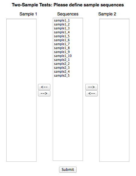
From the interface above user can designate sequences into two groups for comparison.
5.2 Outputs
P values of Z-test and T-test.
6. Sequence clustering
A genetic similarity cluster identification tool that includes two approaches to defining clusters: the first is based on pairwise genetic distance and is algorithmically similar to the approach used by HIV-TRACE (a tool developed by Sergei Kosakovksy Pond and Joel Wertheim, in wide use by the CDC); the second is based on phylogenetic branch lengths and is modified from a tool developed by Art Poon.
6.1 Inputs
6.2 Outputs
Sequence clustering CSV file
Sequence Distance matrix CSV file
Users can retrieve finished results via a previously assigned project id.
1. Lanave, C., Preparata, G., Saccone, C. & G. A. Serio. 1984. New method for calculating evolutionary substitution rates. Journal of Molecular Evolution
20:86-93.
2. Tavare, S. 1986. Some probabilistic and statistical problems on the analysis of DNA sequences. Lectures on Mathematics in the Life Sciences 17:
57-86.
3. Jukes, T. & C. Cantor. 1969. Evolution of protein molecules. In Munro, H. (ed.) Mammalian Protein Metabolism, vol. III, chap. 24, 21-132
(Academic Press, New York).
4. Kimura, M. A. 1980. Simple method for estimating evolutionary rates of base substitutions through comparative studies of nucleotide sequences.
Journal of Molecular Evolution 16:111-120.
5. Felsenstein, J. 1981. Evolutionary trees from DNA sequences: a maximum likelihood approach. Journal of Molecular Evolution 17:368-376.
6. Hasegawa, M., Kishino, H. & T. Yano. 1985. Dating of the Human-Ape splitting by a molecular clock of mitochondrial-DNA. Journal of Molecular
Evolution 22:160-174.
7. Tamura, K. & M. Nei. 1993. Estimation of the number of nucleotide substitutions in the control region of mitochondrial DNA in humans and chimpanzees.
Molecular Biology and Evolution 10:512-526.
8. Le, S. & O. Gascuel. 2008. An improved general amino-acid replacement matrix. Mol. Biol. Evol. 25:1307-1320.
9. Nickle DC, Heath L, Jensen MA, Gilbert PB, Mullins JI, Kosakovsky Pond SL. 2007. HIV-specific probabilistic models of protein evolution.
PLoS ONE 2:e503.
10. Whelan, S. & N. Goldman. 2001. A general empirical model of protein evolution derived from multiple protein families using a maximum-likelihood
approach. Molecular Biology and Evolution 18:691-699.
11. Dayhoff, M., Schwartz, R. & B. Orcutt. 1978. A model of evolutionary change in proteins. In Dayhoff, M. (ed.) Atlas of Protein Sequence and Structure,
vol. 5, 345-352 (National Biomedical Research Foundation, Washington, D. C.).
12. Jones, D., Taylor, W. & J. Thornton. 1992. The rapid generation of mutation data matrices from protein sequences. Computer Applications in the
Biosciences (CABIOS) 8:275-282.
13. Henikoff, S. & J. Henikoff. 1992. Amino acid substitution matrices from protein blocks. Proceedings of the National Academy of Sciences of the
United States of America (PNAS) 89:10915-10919.
14. Adachi, J. & M. Hasegawa. 1996. MOLPHY version 2.3. programs for molecular phylogenetics based on maximum likelihood. In Ishiguro, M. et al. (eds.)
Computer Science Monographs, 28 (The Institute of Statistical Mathematics, Tokyo).
15. Dimmic, M., Rest, J., Mindell, D. & D. Goldstein. 2002. rtREV: an amino acid substitution matrix for inference of retrovirus and reverse
transcriptase phylogeny. Journal of Molecular Evolution 55:65-73.
16. Adachi, J., P., W., Martin, W. & M. Hasegawa. 2000. Plastid genome phylogeny and a model of amino acid substitution for proteins encoded by
chloroplast DNA. Journal of Molecular Evolution 50:348-358.
17. Kosiol, C. & N. Goldman. 2004. Different versions of the Dayhoff rate matrix. Molecular Biology and Evolution 22:193-199.
18. Muller, T. & M. Vingron. 2000. Modeling amino acid replacement. Journal of Computational Biology 7:761-776.
19. Abascal F, Posada D, Zardoya R. 2007. MtArt: a new model of amino acid replacement for Arthropoda. Mol Biol Evol. 24:1-5.
20. Cao, Y. et al. 1998. Conflict among individual mitochondrial proteins in resolving the phylogeny of eutherian orders. Journal of Molecular
Evolution 47:307-322.
21. Yang, Z. 1994. Maximum likelihood phylogenetic estimation from DNA sequences with variable rates over sites: approximate methods.
J Mol Evol. 39:306-14.
22. Guindon, S. & O. Gascuel. 2003. A simple, fast and accurate algorithm to estimate large phylogenies by maximum likelihood. Systematic Biology
52:696-704.
23. Hordijk W. & O. Gascuel. 2005. Improving the efficiency of SPR moves in phylogenetic tree search methods based on maximum likelihood.
Bioinformatics 21:4338-4347.
24. Anisimova M. & O. Gascuel. 2006. Approximate Likelihood-Ratio Test for Branches: A Fast, Accurate, and Powerful Alternative. Systematic Biology,
55:539-552.
25. Stamatakis, A. et al. A rapid bootstrap algorithm for the raxml web servers, Syst. Biol., 2008, 57:758-771.
26. Stamatakis, A. Phylogenetic models of rate heterogeneity: a high performance computing perspective, Proceedings 20th IEEE International Parallel & Distributed Processing Symposium, Rhodes Island, 2006, pp. 8 pp.-.